How To Determine Outliers In Analytical Data
How to Find Outliers In a Data Set
Analytical method validation can be a challenging beast to handle at the best of times, and after all mistakes happen – we are only human after all.
A single erroneous data point can be enough to skew results and cause a validation to fail.
Just one simple mistake in sample preparation for example can lead to hours of wasted sample preparation and instrument run time – a nightmare scenario in any high throughput lab.
Fortunately, this can be easily avoided through careful planning of a method validation. The inclusion of an additional linearity or quality control (QC) sample than the regulated minimum requirement allows for the rejection of the spurious data point with the requirements still met.
But, how exactly do we determine what is and isn’t an outlier? How do we justify the rejection of a suspected spurious data point?
Fear not for an unlikely hero exists – statistics!
There are several statistical tests used throughout the world of analytical chemistry to determine the presence of a single outlier such as the Grubbs1 test and Dixons Q2 test.
In the following example we see how the Dixons Q test can be used to identify and reject an outlier from a set of quality control (QC) samples.
Example of Outlier Rejection Using Dixons Q Test
The following is an example data set of quality control (QC) samples taken from a method validation for an impurity assay. This assay forms part of a submission to EU regulatory bodies for the import of a pesticide or plant protection product (PPP).
These QC samples have been prepared by spiking a known amount of the impurity (20.02 µg/mL) onto 6 independently weighed technical samples. This is equivalent to 0.1% w/w level of the impurity with respect to the active ingredient content. According to the guidance document for pesticide submission in the EU SANCO/3030/99 rev.53 these samples can be used to determine the repeatability and limit of quantification (LOQ) of the impurity.
Within this document (section 4.1.2.) it defines that a minimum of 5 independent weighing’s are required for determining the precision of a method.
In this example 6 samples have been prepared in order to allow for the rejection of a single outlier and still meet the requirements of the validation.
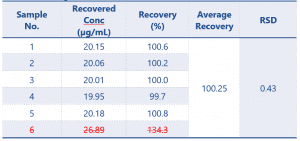
Results for the 6 samples are shown in Table 1, sample number 6 appears to show an obvious spurious result.
Table 1 Initial Results of the QC Samples (n=6)
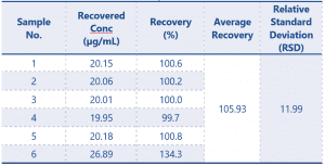
According to the guidance document for this result to be considered acceptable the RSD should be ≤ 5.36 or ≤ 10.72 with a suitable explanation provided. The result of 11.99 would lead to the validation failing.
So, how do we determine if sample 6 is indeed an outlier, and save the day?
The Dixons Q test, first of all we need to find Qexperimental which is calculated as follows:
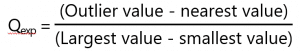
Once we have this value we then need to compare it to the Qcritical value which is determined using a Dixons Q table based on the number of points within the data set.
Table 2 Dixons Q Table
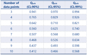
CL refers to confidence limit – that is to say that at CL:90% we can say that the chance of an erroneous rejection of a data point would be 10%.
The most commonly used Qcrit value is at 95% CL, however a lab should define which limit is acceptable for use within their standard operating procedures (SOP).
So, for our example data set the Qexp value would be calculated as follows:
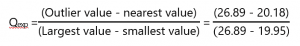
This calculation gives a Qexp value of 0.967.
The number of data points in our data set is n=6 therefore using the Dixons Table our Qcrit value, with a confidence value of 95% is 0.625.
In order for a result to be rejected the test demands that Qexp > Qcrit.
In this example we have calculated a Qexp value of 0.967 which is greater than the Qcrit value of 0.625, therefore we can confidently state that sample number 6 is indeed an outlier and can reject the results from this sample.
With this in mind we can now recalculate our QC sample results with the data points adjusted to n = 5, excluding sample 6.
The recalculated results are shown in Table 3.
Table 3 Final Results of the QC Samples (n=5) – excluding sample 6 as outlier according to Dixons Q
The results of the QC samples at n=5 show a massive improvement on the original calculation, now that the outlier has been removed.
The QC samples now meet the requirements of the guidance document and so the validation will pass.
Conclusion
Statistical tests such as Dixons Q and the Grubbs test are very useful tools which can be easily implemented to determine whether or not a single suspect data point is an outlier.
These tools, along with careful planning of a method validation, can lead to a reduction in the number of repeat assays required, helping to ensure the high throughput your lab requires.
Download Our Guide On Determining Outliers
To download this technical note, click the following link: Determining and Rejecting Outliers in Data
Get In Touch
If you have any questions on the topic, please get in touch, and a member of our team will be happy to help.
Additionally, if you enjoyed this article and wish to keep up to date with our latest news, join us on social media: LinkedIn, Facebook, Twitter.
References
- https://www.itl.nist.gov/div898/handbook/eda/section3/eda35h1.htm Grubbs Test
- https://www.statisticshowto.com/dixons-q-test/ Dixons Q Test
- https://food.ec.europa.eu/system/files/2019-03/pesticides_ppp_app-proc_guide_phys-chem-ana_3030.pdf SANCO/3030/99 rev.5 European Commission, Pesticides, Plant Protection Products, 22 March 2019